GIVING FORMAT
In this lesson, we will learn how to give format to the data we are working with.
To change the font type
1. We shade the area we want to change in format. Remember, to shade, we click and keep the left button of our mouse pressed. We move the mouse to cover the area we want to change.
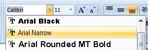
2. In this case, we will change the font style, so we look for this option in the Home tab options.
3. We open up the menu and we select the type of font we want. In this case, we choose Arial Narrow.
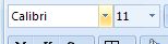
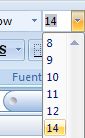
4. We can also change the font size using the number which appears next to the font style.
We open the menu to select the new desired size. For example, we will change the size form 11 to 14. A tip: to open up some menus, we must click on the small arrow.
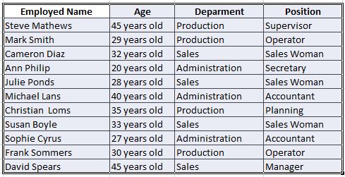
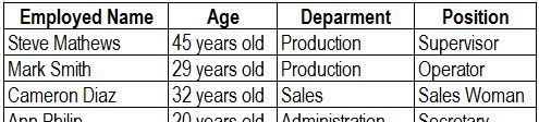
5. Now, our data will have a new format. Lets see a couple of them in the following image:
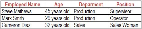
We can also change the font colour:
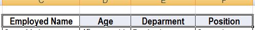
a) We shade the cells we want to change the colour for. We move the cursor over the cell that contains Employee Name. We click and keep the left button on the mouse pressed to shade Age, Department, and Position.
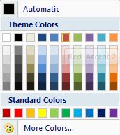
b) We look for the Font Colour option in the Home tab toolbar.

c) We open the options menu and we select the colour we want. In this case, we will choose Red.
d) Now, our parameters are written in that colour. Lets see: