MORE ON EXCEL GRAPHS
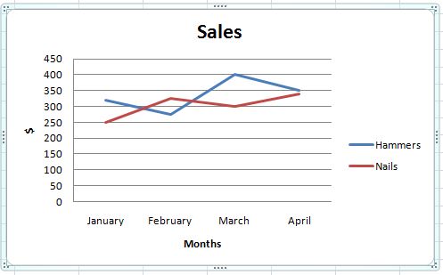
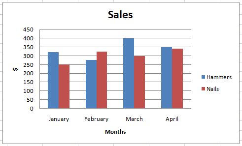
In the previous lesson, we created a column graph using the information on hammers and nails sales between the months of January and April.
We also learnt how to write a title for our graph. We will learn a few more things in this lesson.
Naming the Axis
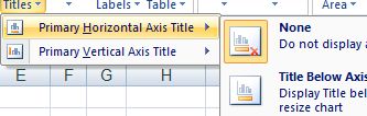
1) We click on the graphic and we select the option Axis Titles from the graphic toolbar.

2) Its options will appear. First, we select Main horizontal axis title, and then, where we want to see this title. For this case, we will choose Title under axis
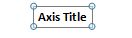
3) In our graphic, a rectangle with the words "Axis title" will appear
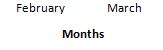
4) We will write the name for the axis in this rectangle, which in this case will be "Months".
5) Then, we click on Axis Headings again and we select Main vertical axis title. For this case, we will choose Rotated Title
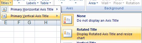
6) In our graph, a rectangle with the words "Axis Title" will appear on the Y-axis.
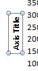
7) In this rectangle, we will write the dollar sign "$", which represents the axis.

8) Lets how our graph looks.
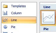
To modify the type of graphic, we click on it and we look for the "Change graphic type" icon in the toolbar.
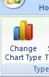
We select the new type of graphic, in this case we will choose a Line graph.
The Graph will have already changed in our worksheet.